City Comfort+ Toolbar Interface

The toolbar contains seven buttons: ‘Project’, ‘Weather’, ‘Topography’, ‘City’, ‘People’, ‘Calculation ‘and ‘Visualization’. Please always follow the operating sequence from left to right. The first five buttons are used to create projects before pressing ‘Calculation’. Results can be loaded using ‘Visualization’. You need to repeat the simulation workflow every time the model is changed.

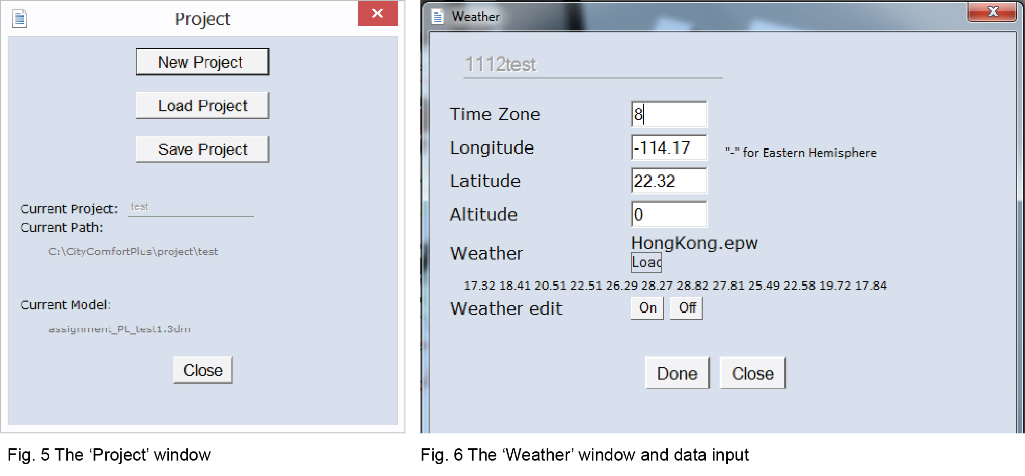
Project: window allows you to ceate a new project or load an existing one. All projects will be saved in C:/CityComfortPlus/project/

Weather: You need to inform CityComfort+ of the location and weather information on the project site. Please key-in the time zone, longitude, latitude and altitude (above sea level). Notice that longitude for the East Hemisphere is negative ‘-‘ and for the Western Hemisphere it is positive ‘+’. The ‘weather’ input accept only .epw file saved locally in your computer. A list of weather file is already present in C:/CityComfortPlus/weather/. Standard weather data in .epw format for 2100+ cities world-wide can be downloaded for free from U.S. Department of Energy (USDOE). If you want to use your own weather data, you need to manually create an .epw file and load it in CityComfort+. An example of the .epw file is provided in Fig. 7.

Topography allows you to define the ground information and sensor grid. You need to follow the command prompt since there is no graphical window.

The first step is to select the terrain, which can be either flat (a plane surface) or hilly (NURBS) of your own input. You are then remained to input the offset of sensor grid above ground. A standard offset is 1.5m above ground, roughly the height of our head/chest where we sense the thermal environment. The last step is to define the range of analysis and input x and y-axis intervals between each sensor grid. After the steps above, a sensor grid will be set up in your model space automatically.

City allows you to define properties of the urban environment. You need to fill in the ‘optical property’, ‘heat island property’ and ‘thermal property’ accordingly.

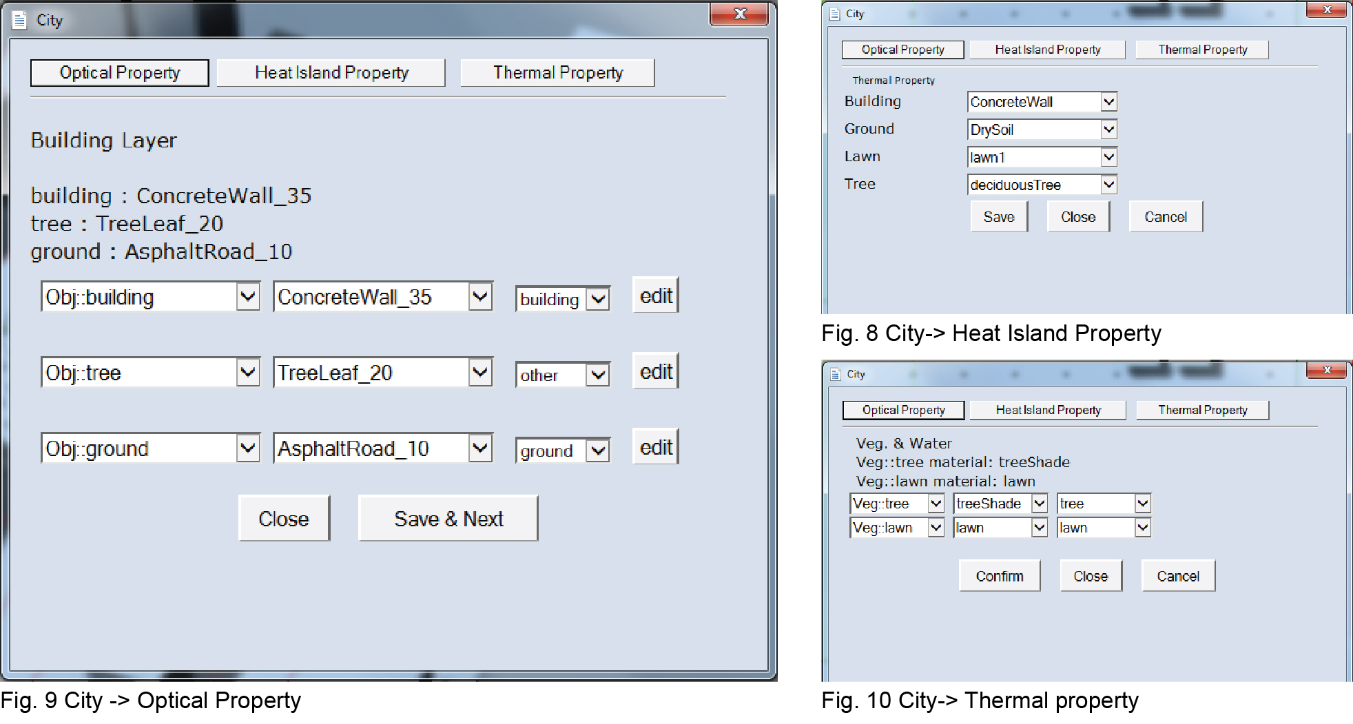
• Optical Property information is needed for all non-transparent objects created under the ‘Obj’ layer. For your convenience, a property library is defined for common urban surfaces such as building walls, ground, or tree leaf. To create customized materials, you need to edit the RADIANCE material library files placed under C:/CityComfortPlus/cfg/. An example is provided in 9.
• Heat Island Property contains additional information required to compute air temperature distributions. Each sub-layer under ‘Veg’ will appear in the list inside the drop-down window and you need to assign material types and values accordingly. An example is provided in 8 where we choose ‘treeShade’ for the Layer ‘tree’ and’ lawn’ for the Layer ‘lawn’. Click Confirm to finish. CityComfort+ will understand an remember your choices.
• Thermal Property requires material input for building, ground, lawn and trees. A library of common materials including concrete, stone, wood, metal, glass, asphalt are provided in the CityComfort+ library. To add new materials, you need to edit the library file of thermalproperty.lib and thermalproperty.map located at C:/CityComfortPlus/library/preload/. After finish this step, click ‘Save’ so that CityComfort+ will store all the information. Click ‘Close’ when finish.

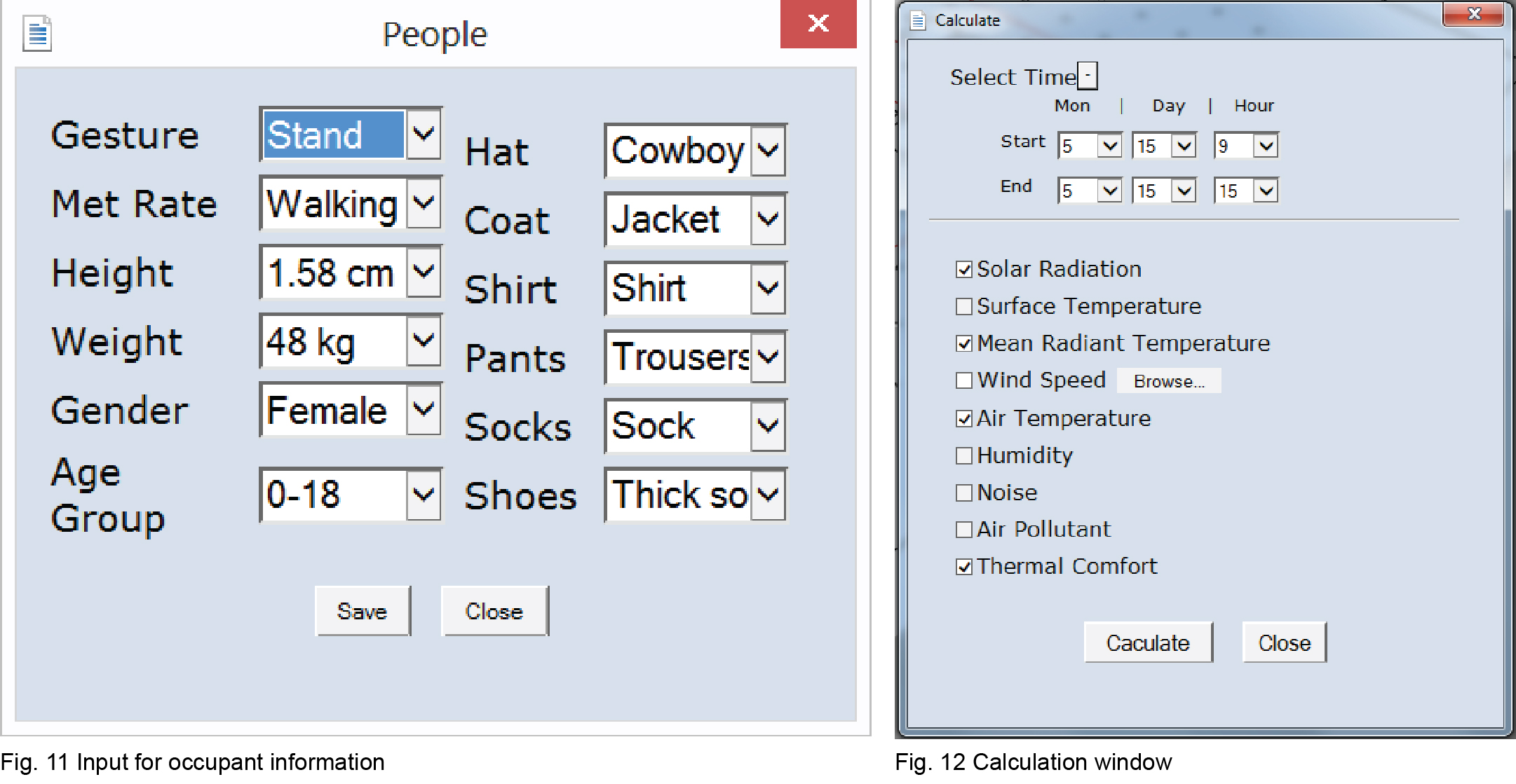
People: Human perception of thermal comfort is closely related to the person condition – bodily gesture, activity level (metabolic rate), height, weight, gender, age, and clothing conditions (Fig. 11). For UTCI metrics, we use a standard walking person with clothing level automatically adjusted based on ambient air temperature and this input is no longer necessary.

Calculation You need to specify the simulation time period and to choose variables to be calculated. Notice that localized wind speed need to be calculated using an external software FlowDesigner 12 and the results in .csv format should be loaded by click the button ‘Browse’.

After you click the ‘Calculate’ button, you will need to manually draw a window on the top-view that covers all site features that matters. The purpose is to allow CityComfort+ to estimate mean building height within 50m radius from each grid point.

The calculation continues afterwards. Click ‘OK’ in all following pop-up windows.

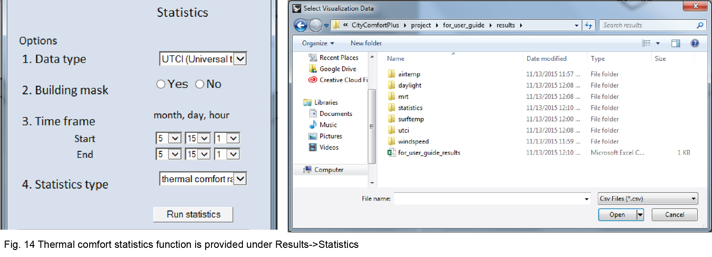
Visualization After finishing the calculation, you can load results in Rhino space. Click the ‘Load’ button and browse the C;/CityComfortPlus/project/yourproject/results/ Variables are located in subfolders such as ‘airtemp’, ‘daylight’, ‘mrt’ (mean radiant temperature), ‘surftemp’, ‘windspeed’ and ‘utci’(Universal Thermal Climate Index). Results are stored in .csv format for each variable and for each hour that you have chosen to calculate. Make sure your current Rhino viewport is ‘Rendered’, and specify the location and the font size for data legend.

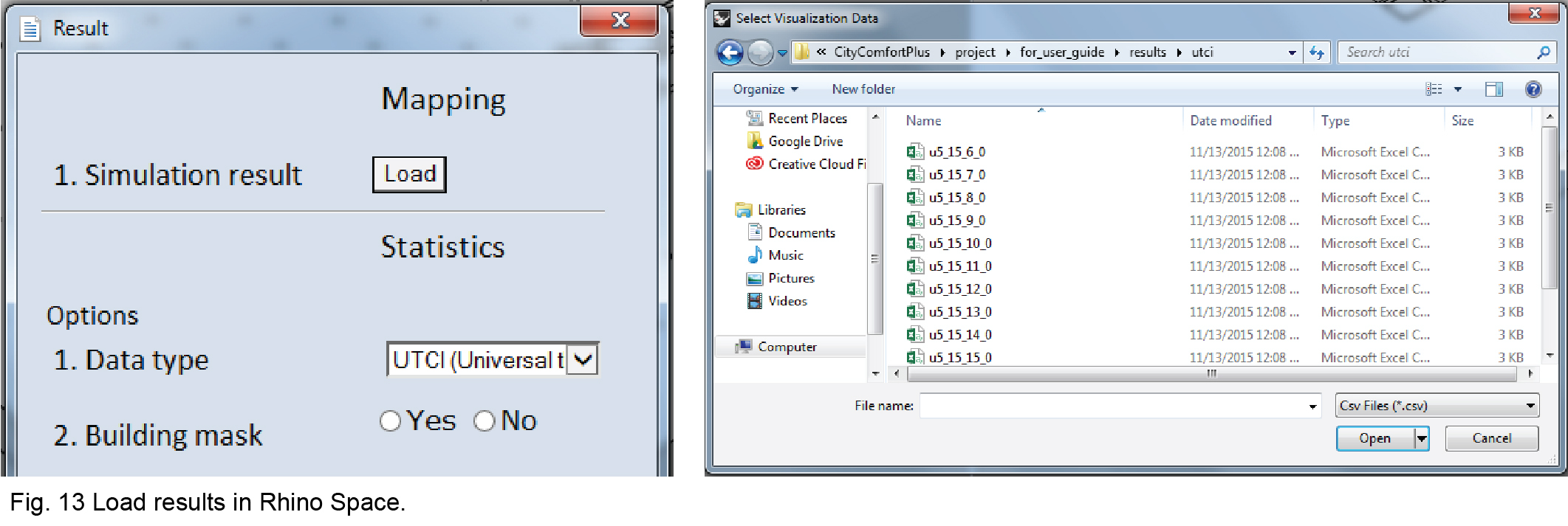
There is a statistical function embedded in CityComfort+ that can compute the accumulative thermal comfort conditions for a designated time period. As it is shown in Fig. 14 Results -> Statistics, chose UTCI, specify the time period needed for statistics, and press ‘Run Statistics’. This will generate statistical results in a subfolder in the following path C:/CityComfortPlus/project/yourprojectname/results/statistics/. The computing of statistics only includes hourly results that are already calculated in previous steps. Otherwise CityComfort+ will ignore those hours that are not calculated beforehand. Example: If your earlier calculation is from 9.am to 3.pm, and select to statistic from 10.am to 2.pm, CityComfort+ can work out the results. But if you select to statistic from 8.am to 1.pm, CityComfort+ will only statistic from 9.am to 1.pm since it could not get the data of 8.am.